Week 5 – Transformer Diagnosis

TL;DR

In the past two curriculum weeks, I have focused on getting my Transformer implementation to its best possible shape.

• Datasets: I ran the transformer on four toy datasets, two sanity-check datasets and a subset of 1 benchmark machine translation dataset.
• Experiments: I ran a set of experiments to understand the effects on weight initialization, weight tying vs. untying, and learning rate schedule on performance, and speed of convergence.
• 16-bit training: I started reading about 16-bit training, and ran some naive experiment to see what kinds of bugs would come up. I will leave this report for the next blog post when the whole exercise will be complete.

Datasets

The four toy datasets are designed to test if the implementation can:

1) transfer signals as-is from the encoder to the decoder, with a symbol copying task. There are 20 symbols, the first two are encoded as <go> and <stop>.

X
[ 1, 18,  3,  6,  6,  2],
[ 1, 15, 13, 14,  7,  2]
Y
[ 1, 18,  3,  6,  6,  2],
[ 1, 15, 13, 14,  7,  2]

2) manipulate the input pattern, with the targets reversed.

X
[ 1, 18,  3,  6,  6,  2],
[ 1, 15, 13, 14,  7,  2]
Y
[ 1,  6,  6,  3, 18,  2],
[ 1,  7, 14, 13, 15,  2]

3) take advantage of additional structure on the input pattern. We should expect the model to converge sooner as it’s easier to remember a fixed sequence ordering and reuse it.

X
[ 1, 15, 16, 17, 18,  2],
[ 1,  8,  9, 10, 11,  2]
Y
[ 1, 15, 16, 17, 18,  2],
[ 1,  8,  9, 10, 11,  2]

4) interpret the symbols as numeric values and perform simple arithmetic on them. For example, predict Y_k as the sum of X_k and X_(k-1).

X
[ 1,  7, 10,  8,  3,  2],
[ 1,  8,  6,  6,  9,  2]
Y
[ 1,  8, 17, 18, 11,  2],
[ 1,  9, 14, 12, 15,  2]

The two sanity-check datasets (Polynomial Expansion, Fake Dates) are also synthetic, and training on them further validate if the transformer can perform more complex reasoning over the entire input context window (instead of a limited local one).

Polynomial Expansion

X
(7-3*z)*(-5*z-9)
(2-2*n)*(n-1)
Y
15*z**2-8*z-63
-2*n**2+4*n-2

Fake Dates

X
april 11 1981
wednesday september 1 2004
Y
1981-04-11
2004-09-01

Finally, I downloaded the WMT-2014 English-French dataset, pushed the data through a byte-pair encoding pipeline, and overfit on a very small subset (Train:1024, Val: 64). I didn’t train on the entire dataset mainly because of compute limitations. It’s also more important for my curriculum to prioritize 16-bit training and image recognition datasets.

X  
<GO> les sché@@ mas et leurs inclu@@ sions sont télé@@ chargés automatiquement depuis internet la première fois qu'ils sont requ@@ is, puis gar@@ dés en cache local@@ ement. <EOS> 
Y
<GO> the schem@@ as and their inclu@@ sions are automatically downloaded once from their internet location, and cach@@ ed loc@@ ally. <EOS>

X
<GO> /@@ 1.1 avec connexions persist@@ antes et compression pour minimiser la charge réseau. <EOS> 
Y
<GO> /@@ 1.1 with persistent connections and compression for minim@@ ising network lo@@ ad. <EOS> 

If the hyperparameters are carefully chosen, the transformer should converge on all these datasets (exact match accuracy at 100% and BLEU > 0.85) within 1-4k steps. The corresponding notebooks are listed here. They follow the same transformer implementation using Heads=2 and N_layers=2, the only difference is the data (look for Dataset, Dataloader and DataModule classes).

• Toy Datasets on symbol copying, reversing, ordering and summation (results covered below)
• Polynomial Expansion with training plots.
• Fake Dates Translation with training plots.
• French-to-English with training plots. (refer to the orange dot for correct BLEU)

Experiments

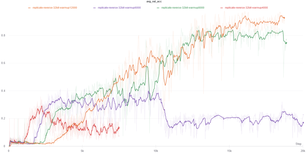
In the process of validating the transformer on the above datasets, I realized that hyperparameters and weight initialization can have substantial effects on convergence and performance. The following plots corresponds to the second toy dataset above (reversing randomly generated input symbols).

Hyperparameter warmup_steps: This hyperparameter directly controls the slope and peak of the learning rate schedule, and it should be adjusted according to the batch size. With a smaller batch size, the weight particles should take smaller steps.

Validation Exact-Match Accuracy (student-forced decoding). Batch size = 100. With low warmup_steps (4000 red, 6000 purple), the learning rate picks up too fast and peaks too high, the weights overstep the minima of the loss surface and never recovered.

Tying / Untying WQKVO at initialization (but not afterwards): For the toy datasets, initializing WQ and WK to the same weights seems important. One possible explanation is that doing so allows the multi-head attention module to start at a sensible baseline that is similar to a simple dot-product attention without linear projections. On the other hand, zeroing out WO was suggested in the Fixup initialization (Zhang et al. 2019) paper for residual learning without any normalization. Our architecture still maintains Layer-Norm between all sub-layers so we don’t see any gains from including this technique.

Validation Exact-Match Accuracy (student-forced decoding). Batch size = 100. With WQ, WK initialized to different weights (i.e. untying, dotted blue), the model’s performance plateaus below 0.4. All other combinations of weight untying verify that this lower performance is indeed due to untying WQ and WK only. Zeroing out WO (solid blue, dotted orange) hurts convergence in our architecture which maintains Layer-Norm.

Embedding Initialization: Because the context length is short(only 8 positions), using sinusoidal embeddings did not benefit training as much as learned embeddings. Once the variance of embedding weights at initialization are scaled by N(0, 1/d_model), rather than the default N(0, 1) set in torch.nn.Embedding, the model converges smoothly at 4k rather than 20k steps. Finally, initializing the learned positional embedding to be N(0, 0.5 * variance of word embeddings) speeds up convergence further by a small margin.

Validation Exact-Match Accuracy (student-forced decoding). Batch size = 100. Sinusoidal positional embeddings (dotted green) are inferior to learned embeddings (all other colors) with short context length(8) on both convergence speed and performance at 20k. Properly scaled N(0, 0.01) embeddings(red, green) converges much faster than N(0, 1) embeddings(purple, grey). Finally, setting the initialization variance of positional embeddings to be half of that of word embeddings improves convergence speed furthermore (red>green, purple>grey).