Week 17 – PMI for Classification; Simple Card Game; Rank Approximation by Dot-products

TL;DR

In the past two weeks, I

realized that point mutual information is a preferable alternative to probability density for zero-shot classification. CLIP is doing the right thing.

rolled back to the original project idea: Studying contrastive learning’s ability to solve compositional problems
- set up a synthetic card game dataset and ran numerical experiments
- found poor rank approximation to be another limitation of dot-product classification

The use of Point Mutual Information in CLIP and GPT-3 predictions

In the last blogpost, I explained that the InfoNCE objective converges $f(x,y)=exp(logit(x,y))$ to $k * \frac{p(x,y)}{p(x)p(y)}$ , and thus using $f(x,y)$ to model $p(x,y)$ or $p(y|x)$ would be inappropriate. While the statement remains valid and results from the corresponding numerical experiments in the last blogpost still support it, using $\frac{p(x,y)}{p(x)p(y)}$ to make predictions is actually preferrable for zero-shot classification.

Imagine we are training a system to identify named entities, and for simplicity, we only care about geographical locations(city, country names). Our training corpus is all of today’s news articles. The locations “new york”, “new england”, “new zealand” are present in the corpus. Suppose a lot happened in New York yesterday, so the bigram count for “new york” is very high in today’s news, while not much has happened in “new england” and “new zealand” so the bigram counts for “new england” and “new zealand” are relatively low. As a results, $p(\texttt{york}|\texttt{new})$ is very high while $p(\texttt{england}|\texttt{new})$ and $p(\texttt{zealand}|\texttt{new})$ are very low. After training our system for a day, we give it a geography test with the following prompt:

Which of the following locations exists in the world?
A. new york
B. new zealand
C. new england
D. new diego
E. new angeles

Answers A, B, C are all valid, so a system that’s good at identifying geography locations should score A, B, C equally high and D, E as zeros. This system should not score A much higher than B and C because of the particular distribution in today’s newspaper. Therefore, it is better to further normalize the scores by the marginal probabilities for “york”, “zealand”, “england”, “diego” and “angeles”. More formally, we only care about the amount of information shared between “new” and each of the five candidates. Therefore, using $\frac{p(x,y)}{p(x)p(y)}$ , which is the exponentiation of point mutual information, is more appropriate when we care about the identification of natural pairings more than the mapping of the particular training distribution.

CLIP was trained using the infoNCE objective, so it naturally normalizes $\frac{p(x,y)}{p(x)p(y)}$ over all the class candidates for zero-shot classification. In fact, GPT-3 also applies a similar correction. The generative model was initially trained to score $p(\texttt{completion},\texttt{context})$ . Therefore, during inference, we expect the system to normalize over all the possible completions to get $p(\texttt{completion}|\texttt{context})$ . However, the researchers applied a correction. They further normalized $p(\texttt{completion}|\texttt{context})$ by the unconditional probability $p(\texttt{completion})$ . Empirically, the GPT-3 model performed better on some datasets with this correction. For details, please refer to section 2.4 in the GPT-3 paper.

Synthetic Card Game Data

I postulate a few basic, reasonable dimensions that quantify the degree of compositionality, including 1) the number of attributes, 2) the number of values, 3) the number of objects, and 4) the number of ways the objects can relate to each other. These dimensions exist by design in datasets like CLEVR, and exist in real-world images as well. My first synthetic dataset’s design exploits the first three dimensions, and it looks a little like the card game SET. The rules are pretty simple:

The query is a pair of cards, each with some attributes:
Query card 1: “red, solid, circle”
Query card 2: “blue, solid, circle”
These two cards share two attributes, “solid” and “circle”, which characterize the query.

These are two example key cards considered as matches:
Key card 1: “green, solid, circle” — matches both query attributes.
Key card 2: “blue, solid, square” — matches only one of the query attributes.

This is an example key card not considered as a match:
Key card 3: “orange, void, square” — matches none of the query attributes

This particular deck has 27 cards with 3 attributes and 3 possible values per attribute:

attributes = { 'color': ['red', 'green', 'blue'], 'fill': ['void', 'dashed', 'solid'], 'shape': ['square', 'circle', 'triangle'] }

A more complex, thicker deck can have 81 cards with 4 attributes and 8 possible values per attribute:

attributes = { 'color': ['red', 'green', 'blue', 'orange', 'cyan', 'magenta', 'black', 'yellow'], 'fill': ['void', 'dashed', 'solid', 'checkered', 'dotted', 'mosaic', 'noise', 'brushed'], 'shape': ['square', 'circle', 'triangle', 'star', 'hexagon', 'pentagon', 'ellipse', 'rectangle'], 'configuration': ['OOO', 'OOX', 'OXO', 'OXX', 'XOO', 'XOX', 'XXO', 'XXX'] }

Interestingly, as we scale up the number of attributes and values per attribute, the distribution matrix (queries along one axis, key along the other axis) representing the matches grows in rank. We are looking at the deck of 27 cards with 3 attributes and 3 values per attribute in the following image. There are 27 cards along the y-axis and 351(27 choose 2) queries along the x-axis. Each bright spot refers to a query-key match. The rank of this matrix is 19.

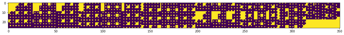
If we scale to 81 cards with 4 attributes and 3 values per attribute. The rank of the matrix grows to 65.

Scaling along the attributes dimension increases the rank rapidly while scaling along the number of values per dimension increases the rank slowly.

Attributes	Values per Attribute	Rank
2	5	9
2	6	11
2	7	13
2	8	15
2	3	5
3	3	19
4	3	65

Approximation of high-rank matrices using dot-product classifiers

In an earlier blog post, I have explained why conventional contrastive learning, which uses a dot-product classifier, may fail to learn highly compositional data due to VC-dimension related reasons. Here, I am suggesting another deficiency of dot-product classifiers.

Following the setup of the card game above, if we try to solve it with a simple contrastive learning model, in which each key is represented as a learnable embedding in $\mathbb{R}^N$ and do the same for each query, each position in the distribution matrix is now approximated by the dot-product between the two corresponding query and key embedding vectors. Zooming out to consider the whole $support(queries)$ by $support(keys)$ distribution matrix $M$ , we are approximating $M$ as $Q^TK$ , where $Q$ is $support(queries)$ by $N$ and $K$ is $support(keys)$ by $N$ . If embedding dimension $N$ is lower than the rank of $M$ , and we continue to shorten it, our model becomes poorer and poorer at approximating the distribution matrix $M$ .

Numerical Validation

Indeed, when we code up this experiment and train the model, we will see that a deck with higher rank requires a larger embedding size to hit 100% accuracy on the training distribution. At the moment, I have a few numerical results with me, but will leave the full report along with other observations for the next blog post.

Share this:

Like this:

Leave a Reply Cancel reply